Is A Hot Dog A Sandwich? Defining the Sandwich with Unsupervised Learning

A Classification of Dough-Wrapped Meats, and a Rigorous Answer to the Hot Dog Problem

Definitional Controversies

What is a sandwich? Apparently, this is a hotly debated topic. If you believe the USDA, a sandwich is “meat or poultry filling between two slices of bread.” This is not the only definition, though.

Here are some common definitions of sandwich, ordered from the strictest to the most permissive:

• “Meat or poultry between two slices of bread” - USDA

• “Two pieces of bread with meat, cheese, or other filling between them, eaten as a light meal” - Google

• “Two or more slices of bread or a split roll having a filling in between” - Merriam Webster (a)

• “One slice of bread covered with food” - Merriam Webster (b)

• “Sandwiches include cold and hot sandwiches of every kind that are prepared and ready to be eaten, whether made on bread, on bagels, on rolls, in pitas, in wraps, or otherwise, and regardless of the filling or number of layers. A sandwich can be as simple as a buttered bagel or roll, or as elaborate as a six-foot, toasted submarine sandwich.” - New York Tax Law

Ham Sandwich — A good test case for “definitely a sandwich.”

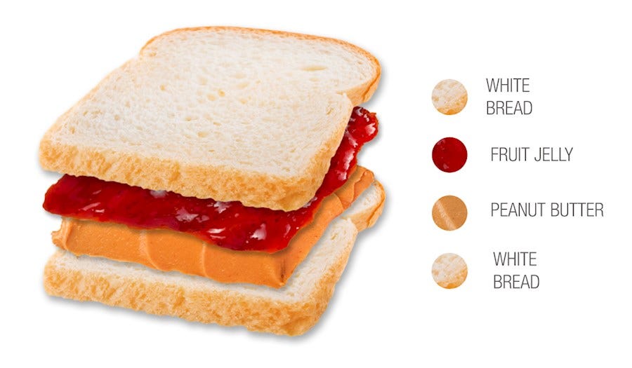
Let’s take the first definition: “meat between two slices of bread.” This definition is obviously nonsense. It excludes, for example, a peanut butter and jelly sandwich, which is an uncontroversial member of the sandwich family. Thus, this definition cannot be right.

In fact, most definitions of “sandwich” seem to run into troubling edge cases. Most frequently, this edge case is the hot dog.

It has some sandwich-like qualities, to be sure.

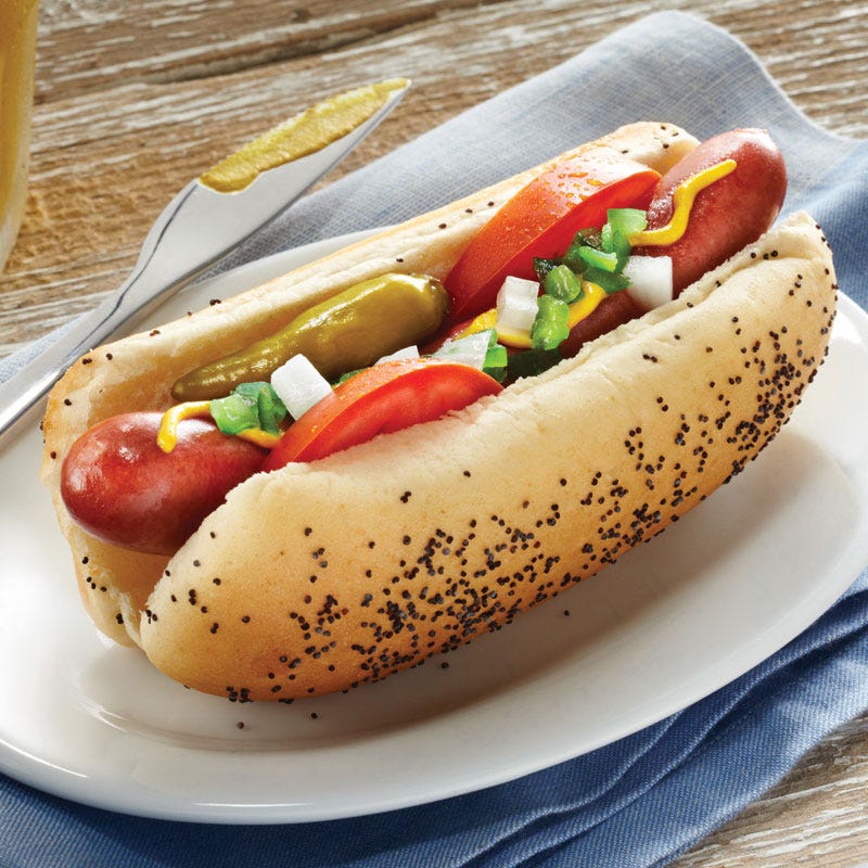
Is the hot dog a sandwich? It certainly has some sandwich-like qualities, but it’s not a clear-cut case of sandwich or not-sandwich. Even Ruth Bader Ginsburg has weighed in on this question (she said yes). No one has yet come to a satisfying conclusion.

---

I claim that everyone is approaching this problem from the wrong direction.

As far as I can tell, every person who’s investigated this question (including New York tax lawyers, the USDA, etc.) has postulated a definition of a sandwich, then tried to justify it by examining test cases within the space of sandwich-like objects. In every case, this approach has failed to produce a universally satisfying definition.

Let us consider how we would teach a computer to identify a sandwich. The obvious approach is some form of supervised learning, where I give a computer examples of sandwiches and not-sandwiches, and train it to tell the difference.

This is known as “supervised” learning because the data set is pre-labeled — I have told the computer what is and is not a sandwich. This is a definition-first approach.

The other type of machine learning is known as unsupervised learning, where a computer learns to recognize patterns in data set without labels.

The simplest example of unsupervised learning is “cluster analysis,” where a computer is taught to group elements into multiple clusters, such that each element within a cluster is more similar to its cluster-mates than to any element of another cluster.

K-means cluster analysis

This is the approach I propose to try. I will construct a data set of various potential sandwich-like objects, label them with their various characteristics (such as bread sweetness, or degree of leavening), and perform unsupervised learning. By doing so, I will discover which features determine the sandwich-ness of any given object. We can then classify objects as more or less sandwich-like in a rigorous fashion, and construct a consistent definition of “sandwich.”

Constructing the Sandwich Data Set

Code and Data Available Here

First, we need examples of sandwich-like foods. This part is easy. Here’s a few:

• Club Sandwich

• Po’ Boy

• Hoagie

• Panini

• Burrito

• Soft Taco

• Hard Taco

• Wrap

• Hot Dog

• Burger

• Calzone

• Pizza

• Cheesesteak

• PB&J

• Oreo

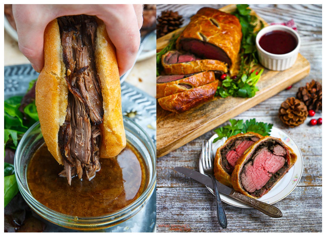
• Beef Wellington

• Grilled Cheese

• And many more

Next, we need some attributes with which to label these potential sandwiches. We want to choose features that stratify our space — ideally, we want our potential sandwiches to form a uniform distribution over each attribute. For example, let’s consider the “number of sides covered by bread” feature.

Number of Sides Covered by Bread, Assuming All Potential Sandwiches are Cubes

If we assume all sandwich-objects are cubic, we can classify them by how many sides are taken up by bread.

In a PB&J, bread covers two sides.

Bread covers two sides

A burrito is trickier. A burrito is not a cube, but the tortilla covers the entire object, and thus let’s call this a full six-sided coverage.

The tortilla covers all (6) sides

The taco is another interesting case. I’m going to say that three sides are covered here.

3 sides covered

A pizza has only one side covered by bread, and so on.

Degree of Bread Leavening

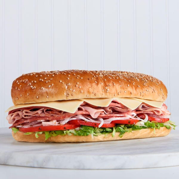
Some things have highly leavened bread, where the bread is very fluffy and soft. Like a hoagie:

A hoagie, or a sub sandwich

Other things have bread which is not leavened at all, like a soft taco:

Some chicken soft tacos

To reduce the number of redundant or unimportant features, I tried to choose features that would partition my sandwiches into reasonably sized groups. For example, the “Deli Meat” category was assigned with the probability that the sandwich-object would contain deli meat. 14/39 examples had a nonzero chance of containing deli meat.

Other features, like “Filling Sweetness” were assigned a number corresponding to the (subjective) sweetness of their filling. Oreo and Ice Cream Sandwiches received a 5, and a French Dip Sandwich received a 0.

Features that only three or four sandwiches shared were discarded as having low predictive power.

The Two Data Sets

I ended up with two data sets. A full data set, containing all the important features I could think of:

Part of the full data set

And a minimal data set, where I removed most of the features, leaving only seven:

• Contains Deli Meat

• Contains Ground Meat

• Contains Raw Tomatoes

• Can Contain Ketchup

• Degree of Bread Leavening

• Number of Sides Covered

• Laminarity (how stacked/layered everything is)

The Minimal Data Set

Classification of Sandwiches Using the Minimal Data Set

Hierarchical Clustering

Code and Data Available Here

First, to check the reasonableness of this data set, I performed hierarchical clustering.

The “bottom-up” or “agglomerative” approach to hierarchical clustering simply finds the two most similar objects, clusters those, and repeats the process until all of the data is within a single cluster.

A visual representation of agglomerative clustering

This produces a family tree where the most similar objects are closest to each other on the tree.

Here’s my family tree of sandwiches represented as a dendrogram:

Hierarchical Sandwich Clustering, performed on the Minimal Data Set

This looks very reasonable! The height of the branch indicates the similarity between the data. For example, dumplings and pasties on the far left are nearly indistinguishable.

A Hot Dog is most similar to a Dirty Dog. Peanut Butter and Jelly has a lot in common with Toast, and a Hoagie and a Po’ Boy are nearly the same thing. There are a couple surprises here, one being that a Meatball Sub is closest to an Empanada. This is probably to do with the paucity of features, and will not be true in the Full Data Set.

With this simple clustering algorithm, we see three distinct clusters emerge. The green cluster contains pretty uncontroversial examples of sandwiches. The red cluster contains both the ultimate example of a sandwich, the Club Sandwich, as well as some questionable sandwiches, such as a hot dog or a wrap. The orange cluster contains no examples of sandwiches, excepting the meatball sub. Interesting!

Principal Component Analysis

Code and Data Available Here

However, we are not after such simplistic classifications of sandwiches. What we desire is a method for classifying an object as sandwich or not-sandwich. A main disadvantage of hierarchical clustering in that respect is that I’ve chosen the descriptive features personally.

For example, it may be that “Contains Raw Tomatoes” is not predictive of sandwich-hood at all. In that case, assigning equal weight to the “Raw Tomatoes” feature as to the “Sides Covered” feature will only confuse our clustering algorithm.

The standard method of assessing the “correct” constellation of features for classifying data is Principal Component Analysis, or PCA. I’ll summarize the key points of that link below.

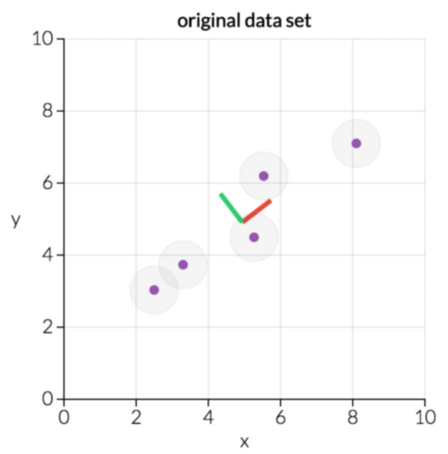
PCA is a “dimensionality-reduction” technique. Suppose I have a data set of five points, with features “x” and “y.” I can plot these points on a graph.

Original Data Set

This is a two-dimensional data set (features x and y), containing five elements. However, it’s pretty clear that this data falls mostly along a line. What happens if I rotate my data set into a new coordinate system?

Rotated Data Set

This is the same data plotted vs. my new axes, called “principal component 1” and “principal component 2.” pc1 and pc2 are new coordinates created from linear combinations of x and y, it looks like pc1 = x + y and pc2 = y - x. The axes are then scaled and moved so the data nicely sits around the origin.

In principal component space, the data falls very nearly along a straight line of constant pc2. Thus, pc2 gives us almost no information about the spread of the data. In fact, if we wanted to reduce our space from two-dimensional to one-dimensional, we can simply ignore pc2 and plot our data entirely against pc1, reducing the dimension of the data while preserving the variance. That’s the key to PCA.

Mathematically, the challenge is to find the correct axes such that the fewest number of principal components explain the largest amount of variance in the data set. Since PCA is a linear method, there is a nice closed form expression for the principal components — the principal components are the eigenvectors of the data covariance matrix. The Wikipedia summary is verbose, but correct, but I like this one by Sebastian Raschka better.

It’s important to note that there are always the same number of principal components as original axes. If you have five features, you have five principal components. The difference is that the principal components are ordered by how much of the data variance they explain, so only the first few principal components are usually important. The rest can be ignored.

Now let’s apply it to sandwiches.

My “Minimal Data Set” has only seven features, and thus is a seven-dimensional data set, with seven principal components. Here are the first two principal components. Again, the principal components are the linear combinations of features that explain the most variance in my data.

PC1 = - 0.48 * Laminarity - 0.42 * Deli Meat - 0.38 * Leavening + …

PC2 = -0.4 * Laminarity + 0.05 * Raw Tomatoes + 0.1 * Sides Covered + …

As you can see, the first two principal components collectively explain ~55% of the variance in my data. This means that we can reduce the dimensionality of the data set from 7 to 2 while losing less than half of the information! This is pretty cool.

Scrutinizing the two principal components, I suspect that PC1 (well, negative PC1) is probably a good definition of “sandwich.” Features with negative weights are “Laminarity,” how stacked the food is, “Presence of Deli Meat,” always a good indicator of a sandwich, “Degree of Bread Leavening,” ruling out foods wrapped in tortillas, etc. Features with positive weights are “Ground Meat,” which isn’t common in sandwiches, and “Sides Covered,” meaning as the food gets more wrapped, it is less of a sandwich. This is a pretty sensible definition. PC2 is much harder to figure out, so let’s plot the sandwiches in my data set vs. the two principal components.

Clustering

Here is the data vs. the first two principal components:

The Minimal Sandwich Data Set in principal component space.

This is quite a reasonable clustering! Note how Hot Dogs, Dirty Dogs, and Pigs-in-a-blanket all cluster up at the top right corner, Club Sandwiches and Reubens are close together, Oreo’s closest neighbor is Ice Cream Sandwich, and a Dumpling and an Empanada are indistinguishable. There’s also some weird features, like Quesadilla being closes to Ice Cream Sandwich in this restricted space, or Egg Salad Sandwich being closest to a Sope.

However, we can’t really cluster these by eye. We are only plotting these sandwiches against the first two principal components, and there are really seven. In order to find the “best” clustering in 7-D space, let’s perform k-means cluster analysis.

K-means clustering is probably the simplest unsupervised learning algorithm. Its purpose is to group points in some abstract space into “clusters” which faithfully represent the areas of high density in the data. The following .gif, taken from this link, gives a pretty good idea of what’s going on:

K-means clustering

I randomly choose k centroids, represented by x in the above gif. I then assign each data point to its closest centroid, forming “clusters.” Then, I find the centroid of each cluster, and move the x to the new centroid. I repeat until convergence. Here’s the pseudo-code from the same link:

K-means clustering algorithm

This algorithm is very simple to implement, and produces reasonable results when clusters are nicely shaped (i.e. ball-like in n dimensions).

There is a deep connection between k-means clustering and principal component analysis. amoeba on the Stats StackExchange says that k-means can be viewed as a super-sparse PCA, and discusses a paper by Ding and He formalizing this notion (though there’s some controversy over whether it is correct). Either way, they can both be seen as attempts to do the same thing — reduce a complex data set to simpler, more meaningful categories, plotted along more meaningful axes.

K-means clustering has one obvious drawback — you need to manually choose the number of clusters with which to partition your data. There are standard methods of choosing K, which the same link goes into in some detail. Fortunately for us, we don’t need to be that rigorous. Let’s run the k-means algorithm on our data set in principal component space and see what comes out.

Let’s look at the K=2 case first:

It’s immediately obvious that the computer agrees with me about PC1 being the “sandwich axis.” The clustering algorithm seems to have put everything with PC1 < 0 in the green cluster, and everything with PC1 > 0 in the red cluster. With the exception of a Wrap, every green dot is an uncontroversial example of a sandwich. For every data point colored red, if you called it a sandwich, someone would yell at you. This very well could represent a consistent definition for “sandwich.”

The K=3 cluster is a little weird. It seems to have identified the partitions in the data well, but its clusters are not obviously meaningful. For example, why are Oreo and Ice Cream Sandwich in different clusters?

K=4 is much better. The blue cluster consists of Hot Dogs and derivatives, Pizza and derivatives, the Sloppy Joe and Meatball Subs, Dumplings, Empanadas, and Baos. This blue cluster could easily be considered the “Ground Meat” cluster. The yellow cluster contains “sandwiches without ketchup,” as in sandwiches where eating them with ketchup would be a crime against food (A PB&J with ketchup, can you imagine?). The green cluster is “sandwiches where ketchup is acceptable,” and the red cluster is a grab bag of whatever is left.

K=5 at first looks nonsensical. Why is that top cluster of Hot Dog, Dirty Dog, and Pig-in-a-Blanket broken up into three distinct clusters? The answer can be found by looking at higher dimensional spaces — recall that we are running k-means clustering on the entire 7-D space of principal components, not just the first two.

Here’s the K=5 clustering plotted against PC1, PC2, PC3, and PC4. You can now see what’s going on. The yellow dots all have high PC4, and the purple dots have low PC4. Here’s a plot of the components of PC3 and PC4.

PC3 seems to ignore laminarity in favor of “ground meat with leavened bread,” i.e. burgers and meatball subs, vs. “Ketchup and Raw Tomatoes.” PC4 is almost entirely dominated by Raw Tomatoes. I’m not sure how meaningful these axes are, and they definitely don’t seem to correlate with sandwich-hood. Let’s ignore them.

The Definition of Sandwich

The K=2 case again

From our K-means analysis, the most informative plot was clearly the K=2 case. We can show algorithmically that foods that we think of as “sandwiches” lie entirely on the left side of the PC1 axis, and foods that are either borderline sandwiches or not-sandwiches lie on the right side. It is natural, therefore, to define a sandwich as something having PC1 < 0. This definition will include a Wrap, which is not traditionally thought of as a sandwich, but has enough sandwich-like qualities to push it over the edge into true sandwich-hood. One of the great advantages to a precise definition is that not only can we define “sandwich,” we can quantify how sandwich-like any given object is.

Thus, from the Minimal Data Set, this is how I define “Sandwich”:

Given:

• D - The probability of containing deli meat

• G - The probability of containing ground meat

• R - The probability of containing raw tomatoes

• K - 1 if ketchup is an acceptable condiment, 0 otherwise

• B - the degree of bread leavening from 0 to 2, with 0 being not leavened and 2 being extremely fluffy

• S - the number of sides covered by the bread or bread-like wrapping, modeling it as a cube

• L - the degree of laminarity or “stack-i-ness,” rated from 0 to 5

Calculate:

PC1 = - 0.452*D + 0.451*G - 0.193*R - 0.295*K - 0.187*B + 0.045*S - 0.101*L

(The coefficients above have been normalized to the maximum value of the suggested scale., i.e. I pre-divided the coefficient of L by 5)

Finally:

A Sandwich is a food with PC1 < 0.

Exercise for the Reader:

Is this food a sandwich? Answer at the bottom of the post.

The Full Data Set

For clarity’s sake, the above analysis uses only seven of the original twenty-five features. The same analysis can be done using the full data set, and is a bit more confusing.

Here’s the initial dendrogram we come up with:

The sandwich family tree is not significantly different from the minimal data set, and is still very reasonable. More nuanced relationships are captured, like the Falafel Pita now being most closely related to the Gyro. In the minimal set the Falafel Pita was most closely related to the Burrito, an odd, though justifiable, choice. The Meatball Sub is no longer the nearest neighbor of the Empanada, being replaced by the much more sensible choice of the Pasty.

Here are the first four principal components of the full data set

PC1 and PC2 of the full data set

PC3 and PC4 of the full data set

We notice immediately that the individual principal components explain less of the variance than before. In the minimal set, two components out of seven was sufficient to explain 55% of the data variance, here we need four out of twenty-five to explain 58% of the variance.

We can again plot the data in principal component space, after doing k-means clustering:

the K=2 clusters from the Full Data Set

The K=2 clustering isn’t nearly as sensible as the minimal data set. Instead, the K=4 clustering is most sensible to me by eye.

the K=4 clusters from the Full Data Set

The blue cluster consists of the “savory” sandwiches, again including the wrap, and the yellow cluster the “sweeter” sandwiches, assuming you count cheese and cream cheese as being “sweet.” Maybe “dairy” sandwiches would be a better classification, though that leaves out PB&J. The green cluster contains the tortilla and less-leavened bread-wrapped foods, and the red cluster contains Hot Dogs, Pizza, Dumplings, and derivatives. The red cluster also contains the French Dip sandwich, which I can only describe as an error, though when you get right down to it, there’s not that much difference between a French Dip and a Beef Wellington.

Unadorned roast beef in bread, served with gravy.

Ultimately, the full data set is more complex to interpret, and probably less useful to our original goal: a consistent and reasonable definition of sandwich. This illustrates a truism in machine learning — sometimes, adding more features makes a worse model.

Concluding Remarks

In this article, we’ve built up a consistent and reasonable definition of sandwich. This is not the only possible definition, and is highly dependent on the data set and the specific chosen features. However, I claim that this method is far more consistent than any of the methods employed by others linked in this post (with the exception of the State of New York, which defines essentially anything as a sandwich).

Thus, we are uniquely equipped to rigorously answer several of the burning questions of our time:

1. Is a Hot Dog a sandwich? No. We find PC1 > 0 for the Hot Dog, and thus reject it as a true member of the sandwich family.

2. How sandwich-like is the Hot Dog? Is PC1 value is quite close to zero, similar to a Falafel Pita or an Ice Cream Sandwich. Thus, it is perhaps best classified as a “pseudo-sandwich.”

3. Why is a Wrap a sandwich? A Wrap contains deli meat, often contains raw tomatoes, and is quite laminar, albeit rolled up in a tortilla. Thus, despite its lack of other sandwich-like qualities, its PC1 value is less than zero. Since its PC1 value is also small, It is perhaps also better classified as a “pseudo-sandwich,” though this is a personal decision.

   

   A Wrap Sandwich. Really.

4. Which constellation of features most clearly delineates a sandwich from a non-sandwich? Objects which are highly laminar, containing deli meat and leavened bread are very likely to be considered sandwiches. Objects with ground meat with more than two sides covered by bread are unlikely to be sandwiches.

And now, to finish off this article, I’m going to go buy a sandwich. For some reason, writing this article made me very hungry.

---

Answer to the exercise posed in The Definition of Sandwich section:

For this object, I calculate PC1 = - 0.452*1 + 0.451*0 - 0.193*1 - 0.295*0 - 0.187*1 + 0.045*1 - 0.101*4 = -1.19. This object, whatever it is, is definitely 100% a sandwich.