How to Fail at Amazon Interviews with Calculus of Variations

Doing a lot of complicated math to avoid a trick question, and an inadvertent tutorial on variational calculus

Mar 11, 2022

The Problem Statement

I came across this supposed Amazon interview question the other day:

https://mindyourdecisions.com/blog/2018/07/12/can-you-solve-amazons-hanging-cable-interview-question/

At first glance, the problem is pretty difficult. In fact, it is pretty difficult. But fortunately, there’s a trick to it.

Now personally, I’m not a huge fan of trick questions. Usually, this is because the “trick” is only one of many possible solutions, and choosing which trick answer is correct is entirely a matter of taste. I especially don’t like trick questions during interviews, unless of course, your job consists of entirely trick questions.

However, I like this particular question for two reasons:

If you notice the trick, it’s pretty cool! An 80 m chain hanging straight down from a 50 m pole will fold into two 40 m halves, with the bottom exactly 10 m above the ground, thus the two poles are 0 m apart.
If you don’t notice the trick, you get to use calculus of variations to solve it, which is probably one of my favorite tools in physics.

In keeping with the theme here at Maximum Effort, Minimum Reward, we’re going to ignore the trick and solve the general problem. After all, how often can you put two poles exactly zero meters apart? Literally never. Let’s solve the general, much more useful case.

Why is this useful? Well, the hanging chain is a critical component of, for example, bridges.

Suspension bridges are made with thick cables hanging under their own weight. The shape that these cables form is thus critically important to the design and construction of the bridge. The shape of the cable is known as a catenary, and all cables hanging under their own weight produce a shape in this family of curves.

A cat-enary is the shape formed by a cat hanging under its own weight

Caveat: Actually doing this amount of math in an Amazon interview is likely to either cause them to hire you on the spot, or immediately reject you for missing the spirit of the problem.

Hanging Chains and Optimization Problems

Solving the Amazon interview question is not straightforward. The question asks “how far apart are the poles?,” but this is not what it’s really asking. It is really asking you to find an expression for the shape of a rope hanging between two fixed points, and the rest of the question follows easily. We can formulate this as an optimization problem using calculus of variations, and then solve it.

Calculus of variations is concerned with maximizing (or minimizing) a functional, which is a function of a function. If that’s not immediately clear, don’t worry, we’ll go through an example.

A hanging chain forms a shape known as a *catenary*.

Consider the hanging chain, of total length L and total mass M. All physical objects act to minimize their potential energy whenever possible. The potential energy U of an object with mass m is U = mgh(x), where g is Earth gravity (9.8 m/s^2) and h(x) is height above the ground at position x.

We can formulate the hanging chain problem as follows: For a chain of length L and mass M with two fixed points a distance d above the ground, find the height of the chain h(x) such that its total potential energy U is minimized.

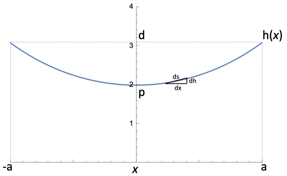
Here’s a better looking diagram for doing math.

A catenary defined by three points. h(0) = p, h(a) = d, h(-a) = d

An infinitesimal section of this chain has length ds and linear mass density M / L. The length ds of this section can be written as:

The total length of the chain L is the integral of ds from x = -a to x = a. This is a constraint on the hanging chain — however it’s hung, it must always have constant length L.

The mass dm = ds * M / L is therefore:

The potential energy of this infinitesimal section is

And thus the total potential energy is:

Mathematically, we can recast our problem as minimizing the functional U[ h(x) ] (U is a function of h(x), and thus a functional) subject to the constraint that the total chain length is L. The output of this optimization problem is a function h*(x), the height of the chain above the ground, that minimizes U[ h(x) ] subject to the constraint

Calculus of Variations Introduction

How do we approach minimization problems such as this? Let’s return to introductory calculus and recall how to minimize a function y(x). A function y(x) is minimized at a “minimizer point” x* when the derivative dy/dx evaluated at x* is zero.

The variation of y is zero at the minimizer point x*

This statement expresses the fundamental concept that near the minimum of y(x), the variation of x does not change y(x).

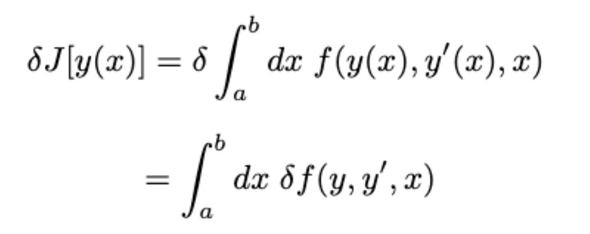
A simple example of finding the minimizer of a function, by setting its derivative to zero.

The idea of something being constant near an extremum can be generalized to functionals. The functional J[ y(x) ] is an integral over some arbitrary function f of y(x), its derivative y’(x), and x:

It is minimized by the “minimizer function” y*(x) when the “variation” of J[ y(x) ] is zero.

The variation of J is zero at the minimizer *y*(x)*

Near the minimizer function y*(x), the variation of y(x) does not change the functional J[y(x)].

Really, calculus of variations is generalizing the concept of the “derivative” to functionals.

What is that delta operator? That’s the “variation” of the functional, and you can think of it as an infinitesimal variation of the path of y(x) by adding small function 𝛿y(x).

First order expression of variation of a functional

y(x) and a small variation 𝛿*y(x),* which is allowed to vary with x

Deriving the Euler-Lagrange Equation

In the case of minimizing a function y(x), we can work through the math and prove that the minimizer point x* must satisfy dy/dx = 0. Let’s work through the same math with the functional J[y(x)].

First we distribute the variational operator 𝛿 through the definition of the functional.

Now, Taylor expanding the expression under the integral sign, and being a bit hand-wavy (don’t worry about the deltas mysteriously turning into partial derivatives, it’s correct)

Distributing variation operator, but changing to partial derivatives

Let’s now consider the second term, proportional to 𝛿y’. We integrate the second term by parts

and notice that 𝛿y(x) on the endpoints a and b is zero by definition, as the endpoints are fixed.

But the variation at the endpoints vanishes

We can plug this new representation back into our expression for the variation of J, finding,

Now, recall the condition for the minimizer y*(x) is 𝛿J[y(x)] = 0.

The “derivative = 0” principle extended to functionals

Since 𝛿y(x) is an arbitrary variation of y(x), the integral expression for 𝛿J[y(x)] is zero if and only if the expression in parentheses is zero.

This is the Euler-Lagrange equation, the fundamental equation of calculus of variations, and the basis of a very large fraction of modern physics.

Euler-Lagrange with Constraints

We’re not quite done though, because what we really want is to solve the hanging chain problem, which has a constraint in it (total length = L).

This constraint is an integral constraint, and is simple to include in our formulation. Consider a general constraint of the form

where L is constant. By the method of Lagrange multipliers we can append this constraint to our functional J[y(x)], forming a new functional K[y(x)] = J[y(x)] + L.

The modified functional, made by adding our constraint to our functional

Let’s think about what we’ve done. The integral of λg is the constant λL, so by appending λg to our integrand, we’ve really just added a constant λL to our functional J. Adding a constant does not affect the location of a minimum or a maximum, but this new functional satisfies an additional constraint! It seems a bit like cheating, but it works. For more detail about constrained optimization, the best reference I have ever found is Donald E. Kirk’s Optimal Control Theory, it’s worth buying a copy of just for Chapter 4 on calculus of variations, but is an excellent book on Control Theory in its own right.

This new augmented integrand fa, which contains our constraint, is also an extremum and must also satisfy the Euler-Lagrange equations, giving us

The constrained Euler-Lagrange equations for fixed endpoints and integral constraint

Solving the Hanging Chain Problem

Armed with all this mathematical machinery, let’s pass our Amazon interview.

We wish to minimize

Explicit expression of potential energy functional for chain

over h(x), subject to

The explicit expression for length constraint of chain

Since multiplicative constants don’t matter for finding an extremum, we can throw out g, M, L, etc, and form our augmented functional

Plugging in to the modified functional expression

and plug the integrand into the Euler-Lagrange equation.

We define our augmented integrand

The Euler-Lagrange equation is

which is a nasty differential equation. In principle, we are now done with this problem — all that remains is to use a powerful symbolic algebra engine to solve the Euler-Lagrange differential equation. However, for extra fun let’s do it explicitly, by hand. Isn’t that fun? I’m honestly not sure anymore.

Sometimes it’s easier to directly integrate the EL equation before plugging in fa, and this is one of those cases. Since our function fa does not explicitly depend on x, multiply through by dh/dx,

The Euler-Lagrange equation, multiplied through by h’(x)

recognize the product rule on the left-hand side of the equation,

Equal to the above equation, but condensed

and finally integrate, forming the first integral of the Euler-Lagrange equation in the case where fa does not explicitly depend on x.

The first integral of the Euler-Lagrange equation for fa which does not explicitly depend on x

This differential equation is simpler and much easier to deal with. We plug in fa and find that the hanging chain must satisfy the following equation.

Our differential equation for the chain height, from the Euler-Lagrange first integral

This differential equation is first order, and separable. Rearranging, we find the following integral

This integral has a standard substitution of h + λ = C cosh(ξ), where cosh is a hyperbolic cosine function, giving us

Simplifying yet further using trig identities, we find

Finally, we integrate and substitute, and we have found the general expression for the shape of a chain hanging under its own weight, the catenary:

Applying Boundary Conditions

We’ve still got some integration constants to take care of, C, D, and the Lagrange multiplier λ.

Returning to our drawing of a catenary, we see we can form three conditions.

Our two boundary conditions, h(0) = p, h(a) = h(-a) = d, and our constraint.

Considering our catenary equation again, we can see the effect of D is to shift the function left and right. Since our catenary is symmetric, we can immediately set D = 0, satisfying the symmetry condition h(a) = h(-a).

We are now in a position to evaluate the length constraint exactly.

Explicit expression for length as a function of *a, C*

Sadly, equations such as this are transcendental, and we cannot evaluate them analytically. Fortunately, we can graph it. Mathematica to the rescue!

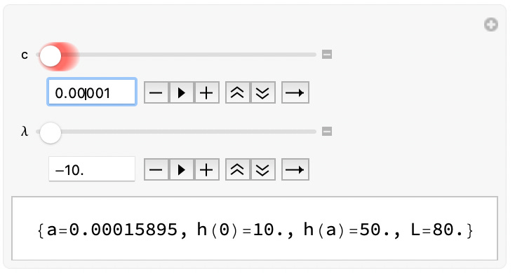
Stephen Wolfram is a bit odd, but Mathematica is awesome

This code allows us to create an interactive plot of the catenary curve. We can vary c and λ (our two undetermined constants) and look at the curves generated.

The x and y axes have very different scales.

Passing our Interview (Finally)?

Now all we have to do is manipulate the constants in the catenary equation until we get the correct answer for the stated problem.

Reproducing the symmetric catenary equation for convenience

This drawing is shown to be *extremely* misleading

In our terminology, what are C, and λ when h(0) = 10 and h(a) = 50? Recall we defined a as the distance from the origin to one of the poles.

A few seconds of moving these sliders around and there we go!

It looks like the constraints we have are satisfied when λ=-10, and we take the limit as c → 0. When we do this, we find that a → 0.

The equation of the Amazon problem! Finally.

The distance between the poles (2a) is zero.

I think I exceeded the 30 minute time limit for our interview. Oh well, I don’t really want to work at Amazon anyway.

If you’ve (somehow) read all the way to the end of this post, thank you. You should comment your accomplishment below. I admit, the cat picture up front was a trap. You draw them in with the cat, then sucker punch them with the calculus. Works every time.

Maximum Effort, Minimum Reward